The BetheŌĆōSalpeter equation (named after Hans Bethe and Edwin Salpeter) [1] describes the bound states of a two-body (particles) quantum field theoretical system in a relativistically covariant formalism. The equation was first published in 1950 at the end of a paper by Yoichiro Nambu, but without derivation. [2]
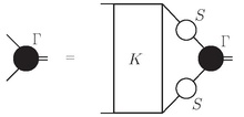
Due to its generality and its application in many branches of theoretical physics, the BetheŌĆōSalpeter equation appears in many different forms. One form, that is quite often used in high energy physics is

where ╬ō is the BetheŌĆōSalpeter amplitude, K the interaction and S the propagators of the two participating particles.
In quantum theory, bound states are objects with lifetimes that are much longer than the time-scale of the interaction ruling their structure (otherwise they are called resonances). Thus the constituents interact essentially infinitely many times. By summing up, infinitely many times, all possible interactions that can occur between the two constituents, the BetheŌĆōSalpeter equation is a tool to calculate properties of bound states. Its solution, the BetheŌĆōSalpeter amplitude, is a description of the bound state under consideration.
As it can be derived via identifying bound-states with poles in the S-matrix, it can be connected to the quantum theoretical description of scattering processes and Green's functions.
The BetheŌĆōSalpeter equation is a general quantum field theoretical tool, thus applications for it can be found in any quantum field theory. Some examples are positronium (bound state of an electronŌĆō positron pair), excitons (bound states of an electronŌĆōhole pairs [3]), and mesons (as quark-antiquark bound states). [4]
Even for simple systems such as the positronium, the equation cannot be solved exactly, although in principle it can be formulated exactly. A classification of the states can be achieved without the need for an exact solution. If one of the particles is significantly more massive than the other, the problem is considerably simplified as one solves the Dirac equation for the lighter particle under the external potential of the heavier particle.
The starting point for the derivation of the BetheŌĆōSalpeter equation is the two-particle (or four point) Dyson equation

in momentum space, where "G" is the two-particle Green function , "S" are the free propagators and "K" is an interaction kernel, which contains all possible interactions between the two particles. The crucial step is now, to assume that bound states appear as poles in the Green function. One assumes, that two particles come together and form a bound state with mass "M", this bound state propagates freely, and then the bound state splits in its two constituents again. Therefore, one introduces the BetheŌĆōSalpeter wave function , which is a transition amplitude of two constituents into a bound state , and then makes an Ansatz for the Green function in the vicinity of the pole as


where P is the total momentum of the system. One sees, that if for this momentum the equation holds, which is exactly the Einstein energy-momentum relation (with the Four-momentum and ), the four-point Green function contains a pole. If one plugs that Ansatz into the Dyson equation above, and sets the total momentum "P" such that the energy-momentum relation holds, on both sides of the term a pole appears.


Comparing the residues yields

This is already the BetheŌĆōSalpeter equation, written in terms of the BetheŌĆōSalpeter wave functions. To obtain the above form one introduces the BetheŌĆōSalpeter amplitudes "╬ō"

and gets finally

which is written down above, with the explicit momentum dependence.

In principle the interaction kernel K contains all possible two-particle-irreducible interactions that can occur between the two constituents. In order to carry out practical calculations one has to model it by choosing a subset of the interactions. As in quantum field theories, interaction is described via the exchange of particles (e.g. photons in quantum electrodynamics, or gluons in quantum chromodynamics), other than contact interactions the most simple interaction is modeled by the exchange of only one of these force-carrying particles with a known propagator.
As the BetheŌĆōSalpeter equation sums up the interaction infinitely many times from a perturbative view point, the resulting Feynman graph resembles the form of a ladder (or rainbow), hence the name of this approximation.
While in quantum electrodynamics (QED) the ladder approximation caused problems with crossing symmetry and gauge invariance, indicating the inclusion of crossed-ladder terms. In quantum chromodynamics (QCD) this approximation is frequently used phenomenologically to calculate hadron mass and its structure in terms of Bethe--Salpeter amplitudes and Faddeev amplitudes, a well-known Ansatz of which is proposed by Maris and Tandy [4]. Such an Ansatz for the dressed quark-gluon vertex within the rainbow-ladder truncation respects chiral symmetry and its dynamical breaking, which therefore is an important modeling of the strong nuclear interaction. As an example the structure of pions can be solved applying the Maris--Tandy Ansatz from the Bethe--Salpeter equation in Euclidean space [5].
As for solutions of any homogeneous equation, that of the BetheŌĆōSalpeter equation is determined up to a numerical factor. This factor has to be specified by a certain normalization condition. For the BetheŌĆōSalpeter amplitudes this is usually done by demanding probability conservation (similar to the normalization of the quantum mechanical wave function), which corresponds to the equation [6]

Normalizations to the charge and energy-momentum tensor of the bound state lead to the same equation. In the rainbow-ladder approximation this Interaction kernel does not depend on the total momentum of the BetheŌĆōSalpeter amplitude, in which case the second term of the normalization condition vanishes.
The Bethe--Salpeter equation applies to all kinematic region of the Bethe--Salpeter amplitude. Consequently it determines the amplitudes where the functions are not continuous. Such singularities are usually located when the constituent momentum is timelike, which are not directly accessible from Euclidean-space solutions of this equation. Instead one develop methods to solve these type of integral equations directly in the timelike region [7]. In the case of scalar bound states through a scalar-particle exchange in the rainbow-ladder truncation, the Bethe--Salpeter equation in the Minkowski space can be solved with the assistance of Nakanishi integral representation [8].
- ABINIT
- ArakiŌĆōSucher correction
- Breit equation
- LippmannŌĆōSchwinger equation
- SchwingerŌĆōDyson equation
- Two-body Dirac equations
- YAMBO code
- ^ H. Bethe, E. Salpeter (1951). "A Relativistic Equation for Bound-State Problems". Physical Review. 84 (6): 1232. Bibcode: 1951PhRv...84.1232S. doi: 10.1103/PhysRev.84.1232.
- ^ Y. Nambu (1950). "Force Potentials in Quantum Field Theory". Progress of Theoretical Physics. 5 (4): 614. doi: 10.1143/PTP.5.614.
- ^ M. S. Dresselhaus; et al. (2007). "Exciton Photophysics of Carbon Nanotubes". Annual Review of Physical Chemistry. 58: 719ŌĆō747. Bibcode: 2007ARPC...58..719D. doi: 10.1146/annurev.physchem.58.032806.104628. PMID 17201684.
- ^ a b P. Maris and P. Tandy (2006). "QCD modeling of hadron physics". Nuclear Physics B. 161: 136. arXiv: nucl-th/0511017. Bibcode: 2006NuPhS.161..136M. doi: 10.1016/j.nuclphysbps.2006.08.012. S2CID 18911873.
- ^ Jia, Shaoyang; Cloët, Ian (2024-02-23), Pion Electromagnetic Form Factor from Bethe-Salpeter Amplitudes with Appropriate Kinematics, doi: 10.48550/arXiv.2402.00285, retrieved 2024-07-31
- ^ N. Nakanishi (1969). "A general survey of the theory of the BetheŌĆōSalpeter equation". Progress of Theoretical Physics Supplement. 43: 1ŌĆō81. Bibcode: 1969PThPS..43....1N. doi: 10.1143/PTPS.43.1.
- ^ Jia, Shaoyang (2017-03-01). "Formulating Schwinger-Dyson Equations for Qed Propagators in Minkowski Space". Dissertations, Theses, and Masters Projects. doi: 10.21220/S2CD44.
- ^ Jia, Shaoyang (2024-02-20). "Direct solution of Minkowski-space Bethe-Salpeter equation in the massive Wick-Cutkosky model". Physical Review D. 109 (3): 036020. doi: 10.1103/PhysRevD.109.036020.
Many modern quantum field theory textbooks and a few articles provide pedagogical accounts for the BetheŌĆōSalpeter equation's context and uses. See:
- W. Greiner, J. Reinhardt (2003). Quantum Electrodynamics (3rd ed.). Springer. ISBN 978-3-540-44029-1.
- Z.K. Silagadze (1998). "WickŌĆōCutkosky model: An introduction". arXiv: hep-ph/9803307.
Still a good introduction is given by the review article of Nakanishi
- N. Nakanishi (1969). "A general survey of the theory of the BetheŌĆōSalpeter equation". Progress of Theoretical Physics Supplement. 43: 1ŌĆō81. Bibcode: 1969PThPS..43....1N. doi: 10.1143/PTPS.43.1.
For historical aspects, see
- E.E. Salpeter (2008). "BetheŌĆōSalpeter equation (origins)". Scholarpedia. 3 (11): 7483. arXiv: 0811.1050. Bibcode: 2008SchpJ...3.7483S. doi: 10.4249/scholarpedia.7483. S2CID 32913032.
- Yambo - plane-wave pseudopotential
- BerkeleyGW ŌĆō plane-wave pseudopotential
- ExC - plane-wave pseudopotential
- Fiesta - Gaussian all-electron
- Abinit - plane-wave pseudopotential
- VASP - plane-wave pseudopotential
For a more comprehensive list of first principles codes see here: List_of_quantum_chemistry_and_solid-state_physics_software
The BetheŌĆōSalpeter equation (named after Hans Bethe and Edwin Salpeter) [1] describes the bound states of a two-body (particles) quantum field theoretical system in a relativistically covariant formalism. The equation was first published in 1950 at the end of a paper by Yoichiro Nambu, but without derivation. [2]
Due to its generality and its application in many branches of theoretical physics, the BetheŌĆōSalpeter equation appears in many different forms. One form, that is quite often used in high energy physics is
where ╬ō is the BetheŌĆōSalpeter amplitude, K the interaction and S the propagators of the two participating particles.
In quantum theory, bound states are objects with lifetimes that are much longer than the time-scale of the interaction ruling their structure (otherwise they are called resonances). Thus the constituents interact essentially infinitely many times. By summing up, infinitely many times, all possible interactions that can occur between the two constituents, the BetheŌĆōSalpeter equation is a tool to calculate properties of bound states. Its solution, the BetheŌĆōSalpeter amplitude, is a description of the bound state under consideration.
As it can be derived via identifying bound-states with poles in the S-matrix, it can be connected to the quantum theoretical description of scattering processes and Green's functions.
The BetheŌĆōSalpeter equation is a general quantum field theoretical tool, thus applications for it can be found in any quantum field theory. Some examples are positronium (bound state of an electronŌĆō positron pair), excitons (bound states of an electronŌĆōhole pairs [3]), and mesons (as quark-antiquark bound states). [4]
Even for simple systems such as the positronium, the equation cannot be solved exactly, although in principle it can be formulated exactly. A classification of the states can be achieved without the need for an exact solution. If one of the particles is significantly more massive than the other, the problem is considerably simplified as one solves the Dirac equation for the lighter particle under the external potential of the heavier particle.
The starting point for the derivation of the BetheŌĆōSalpeter equation is the two-particle (or four point) Dyson equation
in momentum space, where "G" is the two-particle Green function , "S" are the free propagators and "K" is an interaction kernel, which contains all possible interactions between the two particles. The crucial step is now, to assume that bound states appear as poles in the Green function. One assumes, that two particles come together and form a bound state with mass "M", this bound state propagates freely, and then the bound state splits in its two constituents again. Therefore, one introduces the BetheŌĆōSalpeter wave function , which is a transition amplitude of two constituents into a bound state , and then makes an Ansatz for the Green function in the vicinity of the pole as
where P is the total momentum of the system. One sees, that if for this momentum the equation holds, which is exactly the Einstein energy-momentum relation (with the Four-momentum and ), the four-point Green function contains a pole. If one plugs that Ansatz into the Dyson equation above, and sets the total momentum "P" such that the energy-momentum relation holds, on both sides of the term a pole appears.
Comparing the residues yields
This is already the BetheŌĆōSalpeter equation, written in terms of the BetheŌĆōSalpeter wave functions. To obtain the above form one introduces the BetheŌĆōSalpeter amplitudes "╬ō"
and gets finally
which is written down above, with the explicit momentum dependence.
In principle the interaction kernel K contains all possible two-particle-irreducible interactions that can occur between the two constituents. In order to carry out practical calculations one has to model it by choosing a subset of the interactions. As in quantum field theories, interaction is described via the exchange of particles (e.g. photons in quantum electrodynamics, or gluons in quantum chromodynamics), other than contact interactions the most simple interaction is modeled by the exchange of only one of these force-carrying particles with a known propagator.
As the BetheŌĆōSalpeter equation sums up the interaction infinitely many times from a perturbative view point, the resulting Feynman graph resembles the form of a ladder (or rainbow), hence the name of this approximation.
While in quantum electrodynamics (QED) the ladder approximation caused problems with crossing symmetry and gauge invariance, indicating the inclusion of crossed-ladder terms. In quantum chromodynamics (QCD) this approximation is frequently used phenomenologically to calculate hadron mass and its structure in terms of Bethe--Salpeter amplitudes and Faddeev amplitudes, a well-known Ansatz of which is proposed by Maris and Tandy [4]. Such an Ansatz for the dressed quark-gluon vertex within the rainbow-ladder truncation respects chiral symmetry and its dynamical breaking, which therefore is an important modeling of the strong nuclear interaction. As an example the structure of pions can be solved applying the Maris--Tandy Ansatz from the Bethe--Salpeter equation in Euclidean space [5].
As for solutions of any homogeneous equation, that of the BetheŌĆōSalpeter equation is determined up to a numerical factor. This factor has to be specified by a certain normalization condition. For the BetheŌĆōSalpeter amplitudes this is usually done by demanding probability conservation (similar to the normalization of the quantum mechanical wave function), which corresponds to the equation [6]
Normalizations to the charge and energy-momentum tensor of the bound state lead to the same equation. In the rainbow-ladder approximation this Interaction kernel does not depend on the total momentum of the BetheŌĆōSalpeter amplitude, in which case the second term of the normalization condition vanishes.
The Bethe--Salpeter equation applies to all kinematic region of the Bethe--Salpeter amplitude. Consequently it determines the amplitudes where the functions are not continuous. Such singularities are usually located when the constituent momentum is timelike, which are not directly accessible from Euclidean-space solutions of this equation. Instead one develop methods to solve these type of integral equations directly in the timelike region [7]. In the case of scalar bound states through a scalar-particle exchange in the rainbow-ladder truncation, the Bethe--Salpeter equation in the Minkowski space can be solved with the assistance of Nakanishi integral representation [8].
- ABINIT
- ArakiŌĆōSucher correction
- Breit equation
- LippmannŌĆōSchwinger equation
- SchwingerŌĆōDyson equation
- Two-body Dirac equations
- YAMBO code
- ^ H. Bethe, E. Salpeter (1951). "A Relativistic Equation for Bound-State Problems". Physical Review. 84 (6): 1232. Bibcode: 1951PhRv...84.1232S. doi: 10.1103/PhysRev.84.1232.
- ^ Y. Nambu (1950). "Force Potentials in Quantum Field Theory". Progress of Theoretical Physics. 5 (4): 614. doi: 10.1143/PTP.5.614.
- ^ M. S. Dresselhaus; et al. (2007). "Exciton Photophysics of Carbon Nanotubes". Annual Review of Physical Chemistry. 58: 719ŌĆō747. Bibcode: 2007ARPC...58..719D. doi: 10.1146/annurev.physchem.58.032806.104628. PMID 17201684.
- ^ a b P. Maris and P. Tandy (2006). "QCD modeling of hadron physics". Nuclear Physics B. 161: 136. arXiv: nucl-th/0511017. Bibcode: 2006NuPhS.161..136M. doi: 10.1016/j.nuclphysbps.2006.08.012. S2CID 18911873.
- ^ Jia, Shaoyang; Cloët, Ian (2024-02-23), Pion Electromagnetic Form Factor from Bethe-Salpeter Amplitudes with Appropriate Kinematics, doi: 10.48550/arXiv.2402.00285, retrieved 2024-07-31
- ^ N. Nakanishi (1969). "A general survey of the theory of the BetheŌĆōSalpeter equation". Progress of Theoretical Physics Supplement. 43: 1ŌĆō81. Bibcode: 1969PThPS..43....1N. doi: 10.1143/PTPS.43.1.
- ^ Jia, Shaoyang (2017-03-01). "Formulating Schwinger-Dyson Equations for Qed Propagators in Minkowski Space". Dissertations, Theses, and Masters Projects. doi: 10.21220/S2CD44.
- ^ Jia, Shaoyang (2024-02-20). "Direct solution of Minkowski-space Bethe-Salpeter equation in the massive Wick-Cutkosky model". Physical Review D. 109 (3): 036020. doi: 10.1103/PhysRevD.109.036020.
Many modern quantum field theory textbooks and a few articles provide pedagogical accounts for the BetheŌĆōSalpeter equation's context and uses. See:
- W. Greiner, J. Reinhardt (2003). Quantum Electrodynamics (3rd ed.). Springer. ISBN 978-3-540-44029-1.
- Z.K. Silagadze (1998). "WickŌĆōCutkosky model: An introduction". arXiv: hep-ph/9803307.
Still a good introduction is given by the review article of Nakanishi
- N. Nakanishi (1969). "A general survey of the theory of the BetheŌĆōSalpeter equation". Progress of Theoretical Physics Supplement. 43: 1ŌĆō81. Bibcode: 1969PThPS..43....1N. doi: 10.1143/PTPS.43.1.
For historical aspects, see
- E.E. Salpeter (2008). "BetheŌĆōSalpeter equation (origins)". Scholarpedia. 3 (11): 7483. arXiv: 0811.1050. Bibcode: 2008SchpJ...3.7483S. doi: 10.4249/scholarpedia.7483. S2CID 32913032.
- Yambo - plane-wave pseudopotential
- BerkeleyGW ŌĆō plane-wave pseudopotential
- ExC - plane-wave pseudopotential
- Fiesta - Gaussian all-electron
- Abinit - plane-wave pseudopotential
- VASP - plane-wave pseudopotential
For a more comprehensive list of first principles codes see here: List_of_quantum_chemistry_and_solid-state_physics_software